Logistic Regression

The logistic regression model is also one of the most popular models in machine learning for performing classification ( predicting the values of a qualitative variable based on predictors ). It is a parametric technique - the model must find the best parameters based on the data -.

This technique is used to adjust the relationship between a qualitative variable $Y$ ( dependent variable ) and a set of predictors $x_1, x_2, ... x_n$ - independent variables - which must be quantitative variables or qualitative variables transformed into quantitative variables ( one-hot encoding or discrete variable digitization ).

The operation of logistic regression is almost identical to linear regression except that it uses a sigmoid function. Like linear regression, we assume that $x$ and $y$ are dependent, meaning that knowing the values of $x$ improves the knowledge of the values of $y$. Therefore, there is a correlation between $x$ and $y$ - as a reminder : the more a variable $x$ is correlated ( positively or negatively ) with the variable $y$, the more important it is for our model because we say it is « discriminant ». – see ( correlation ).

Logistic regression does not directly predict a qualitative value but a probability that a new record belongs to a class.

Linear vs Logistic

When we talk about regression, it refers to any process that tends to find relationships between variables.

Linear regression seeks to establish a linear relationship between the dependent variable (y) and the explanatory or independent variables $x$ ($x_1, x_2, x_3, ..., x_n$) ( predictors ). Example of simple linear regression : if the car’s age increases by 1 year, the price will be impacted by $z$ ( according to the coefficient and the origin of the line ).

Logistic regression also seeks to establish a relationship between the dependent variable (y) and the explanatory or independent variables $x$ ($x_1, x_2, x_3, ..., x_n$) ( predictors ) but uses a logistic function ( logit ) to obtain a value between $0$ and $1$, which is the probability that a new record belongs to a class. For example, if the car’s age increases by 1 year, the probability that it breaks down will increase or decrease depending on the coefficient associated with age in the model.

One uses a linear function while the other uses a sigmoid function which, through an underlying linear function, models a probability.

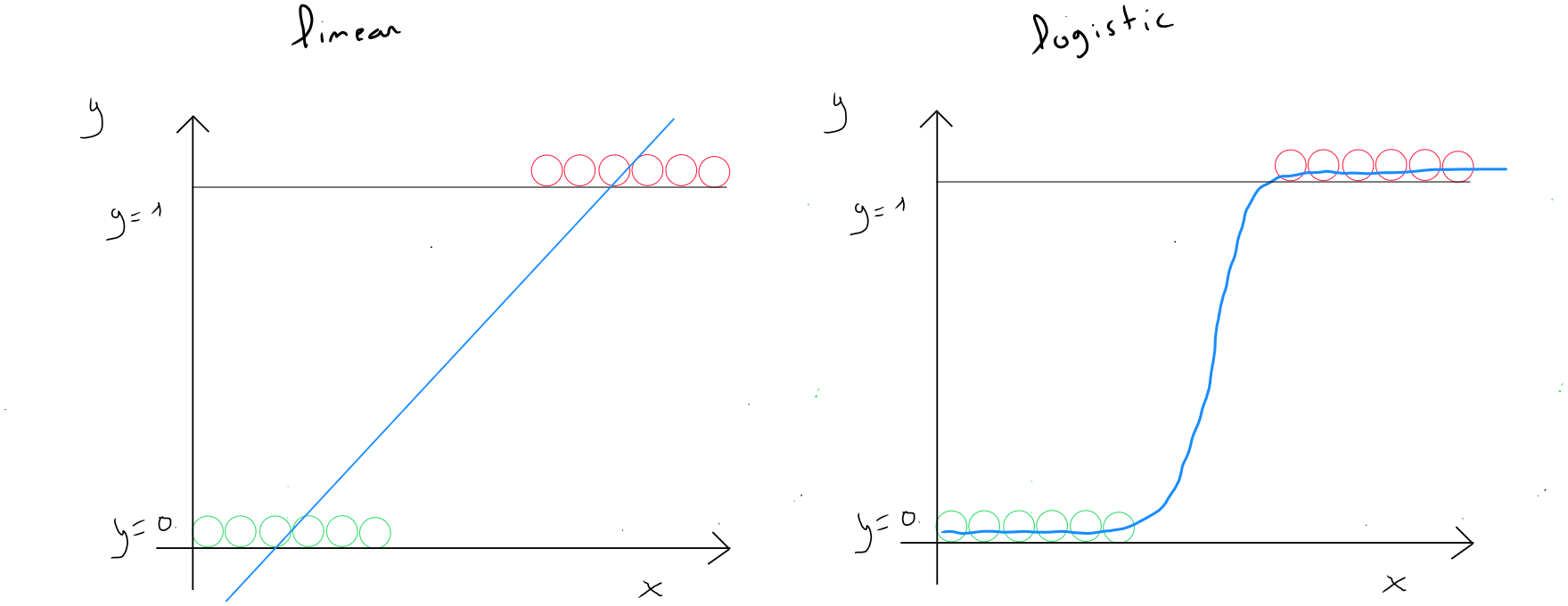
Why Not Use Linear Regression ?

Let’s take the example of a classification with two values : $y = 1$ or $y = 0$. We have a distribution of values for both cases. If we use linear regression and draw the line, we could, in the example illustrated below on the left, consider that linear regression does a correct job, assuming we define a threshold of 0.5 to say that any value equal to or greater than $0.5$ equals $1$ ( class 1 ) and any value below $0.5$ equals $0$ ( class $0$ ). We see in the left graph that all values to the right of the perpendicular to $x$ have a threshold greater than or equal to $0.5$ and thus $1$.

If suddenly, we have a record where the value of $x$ is much higher ( right graph – purple dot ), in this case, the slope of the line is modified, and we see that the model would predict some values greater than or equal to the $0.5$ threshold as belonging to class $0$.

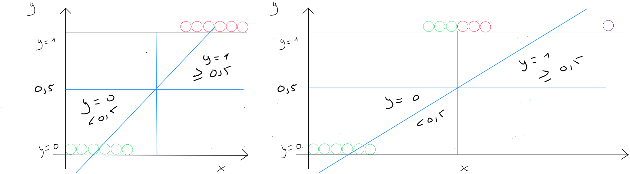
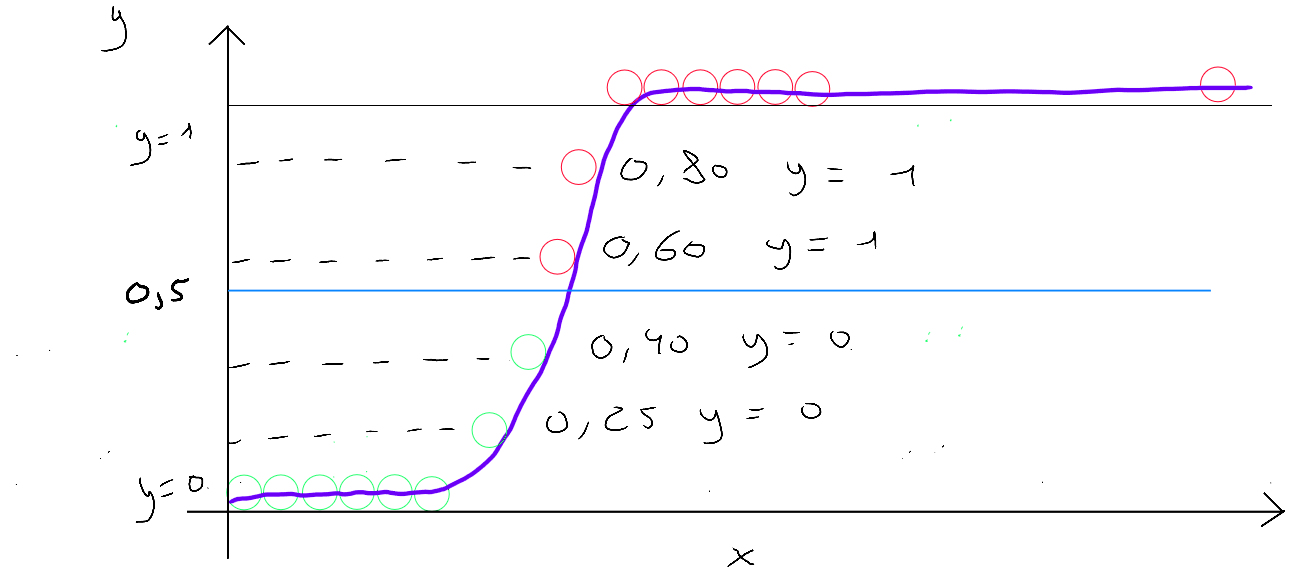
Therefore, we need to use a function that allows us to obtain a curve with the particularity of applying a linear form in a sub-function when values increase exponentially, but that would be flat at the beginning and end so that the values always remain between $0$ and $1$. Specifically, it is an S-shaped function to ensure that possible values are between $0$ and $1$.

$$\begin{aligned} \text{Si } f_{w,b}(x) &\geq 0.5 \rightarrow \hat{y} = 1\\ \text{Si } f_{w,b}(x) &< 0.5 \rightarrow \hat{y} = 0 \end{aligned}$$

Sigmoid Function

The sigmoid function - logistic function - is an S-shaped mathematical function that transforms any value into a number between $0$ and $1$.

$$f(z) = \frac{1}{1 + e^{(-z)}}$$

or

$$z = \vec{w} \cdot \vec{x} + b$$

$Z$ represents the linear sub-function. Just like linear regression, the logistic regression algorithm has training data, i.e. $x$ and $y$, and based on this information, it must identify the parameters $w,b$ through a cost function and the gradient descent algorithm to find the local optimum. Once the parameters are identified, the sigmoid model outputs a value between 0 and 1 – a probability – which is transformed into a class based on a threshold definition ( usually $0.5$ ).

When rewritten in detail, the formula for $z$ gives us this :

$$Z = b + w_1 x_1^{(i)} + w_2 x_2^{(i)} + w_3 x_3^{(i)} + ... + w_p x_p^{(i)}$$

and therefore the formula for the sigmoid function :

$$f(z) = \frac{1}{1 + e^{(-z)}} = \frac{1}{1 + e^{(-(b + w_1 x_1^{(i)} + w_2 x_2^{(i)} + w_3 x_3^{(i)} + ... + w_p x_p^{(i)}))}}$$

or

$$f(z) = \frac{1}{1 + e^{(-z)}} = \frac{1}{1 + e^{(-(\vec{w} \cdot \vec{x} + b))}}$$

If we break down the formula :

• $f(z)$ is the output of the sigmoid function, which gives us a value between $0$ and $1$ ;
• $z$ is the input to the function - which contains the parameters identified by the gradient descent algorithm based on the training data -. $z$ also requires new values of $x$ to predict a probability ;
• $e$ is Euler’s constant ( approximate value of $2.71828$ ) and plays a crucial role in obtaining the S-shape ;

warning

No matter the value of $Z$, the negative exponent of Euler's constant in the denominator will ensure that :

• if $Z$ is a very large positive value $( +∞ )$, the sigmoid function will approach a maximum of $1$ ;
• if $Z$ is a very large negative value $( -∞ )$, the sigmoid function will approach a minimum of $0$ ;

Sigmoid function in Python

def sigmoid(z):
    g = 1/(1+np.exp(-z))
    return g

# (z = np.dot(X[i],w)+b) - define later in the cost function

Decision Threshold

Logistic regression allows us to output a value between $0$ and $1$ from the function $f$, and we, as data scientists, must define the threshold for class $1$ or class $0$. In the literature, the threshold of $0.5$ is often mentioned, such that if the prediction value is $>= 0.5$, then $\hat{y} = 1$, and if the prediction value is $< 0.5$, then $\hat{y} = 0$.

Linear Threshold

In the case of a linear decision based on two predictors ( $x_1, X_2$ ), we could represent the data as follows (diagram below) for values where $z = \vec{w} \cdot \vec{x} + b$, which corresponds to $z = w_1 \cdot x_1 + w_2 \cdot x_2 + b$

To simplify the example, let's define 1 for $w_1$ and $w_2$, and -3 for $b$.

The linear decision threshold in this case would correspond to the moment when : $z = \vec{w} \cdot \vec{x} + b = 0$ as this threshold would be neutral in defining whether $y = 1$ (red cross) or $y = 0$ (blue circle).

In our case, since $w_1$ and $w_2$ are both 1 and $b$ is -3, we can rewrite the equation as follows : $z = x_1 + x_2 - 3 = 0$ . Therefore, $x_1 + x_2 = 3$.

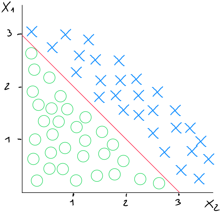
The formula for the linear decision threshold corresponds to the initial formula for logistic regression :

$$f(z) = \frac{1}{1 + e^{(-z)}}$$

or

$$z = \vec{w} \cdot \vec{x} + b$$

Non-Linear Threshold

As we discussed for polynomial regression in the chapter on linear regression, we may encounter cases in logistic regression where the data separation is non-linear.

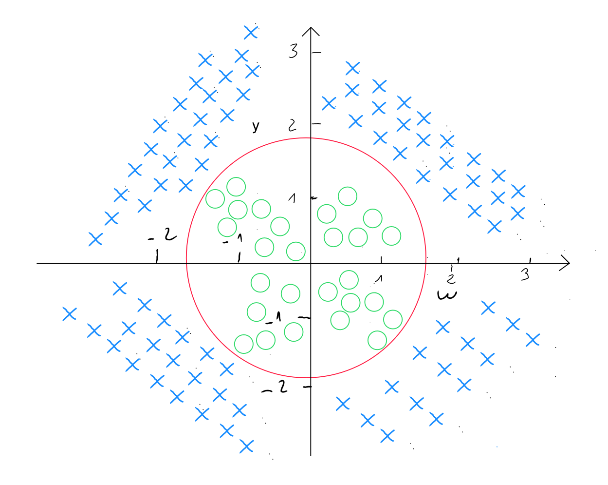
In the case of a non-linear threshold, we will use polynomial features by adapting the formula as follows ( for two predictors $x_1$ and $x_2$) :

$$z = w_1*x_1 + w_2*x_2 + w_3*x_1^2 + w_4*x_1*x_2 + w_5*x_2^2 + .... + b$$

or

$$f(z) = \frac{1}{1 + e^{(-(w_1*x_1 + w_2*x_2 + w_3*x_1^2 + w_4*x_1*x_2 + w_5*x_2^2 + b ))}}$$

Other degrees of polynomial forms are, of course, tested within the algorithm to find the best way to predict the information. For example, in the following cases :

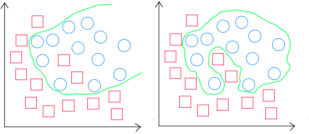
The equation would take the following form :

$$z = w_1 \cdot x_1 + w_2 \cdot x_2 + w_3 \cdot x_1^2 + w_4 \cdot x_1 \cdot x_2 + w_5 \cdot x_2^2 + w_6 \cdot x_1^3 + \dots + b$$

Polynomial function in Python (Non-linear threshold)

import numpy as np
import pandas as pd
from sklearn.preprocessing import PolynomialFeatures, StandardScaler
from sklearn.model_selection import train_test_split
import math, copy
from sklearn.metrics import confusion_matrix

# Data split
data = pd.read_csv('data.csv')

# Variables split
x = data[['x_1', 'x_2', 'x_3', 'x_4', 'x_5', '...', 'x_n']].values  
y = data['y'].values  

# Generation of 3rd Degree Polynomial Terms
poly = PolynomialFeatures(degree=3)
x_poly = poly.fit_transform(x)

# Standardization of Polynomial Data
scaler_x = StandardScaler()
x_poly = scaler_x.fit_transform(x_poly)

# Splitting into Training and Test Sets

x_train, x_test, y_train, y_test = train_test_split(x_poly, y, test_size=0.4, random_state=42)

Cost Function

The shape of the cost function in linear regression is convex, which is optimal for the gradient descent algorithm, whose goal is - through iteration -to find the optimal values for $w$ and $b$.

In linear regression, we use the following formula for the cost function : $J(\vec{w}, b) = \frac{1}{2m} \sum_{i=1}^m \left( (\vec{w} \cdot \vec{x}^{(i)} + b) - y^{(i)} \right)^2$ The objective is then to find the parameters that minimize this cost, $\min_{w,b} J(w,b)$.

The problem with logistic regression is that the shape of its cost function is non-convex, meaning that gradient descent can find several local optima that may not correspond to the true minimum $min J(w,b)$ and can get stuck in convergence.

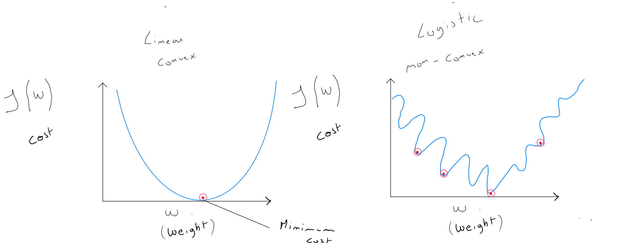
Logistic regression uses a « transformed » cost function from linear regression to make the cost function convex again, allowing it to converge towards a local optimum.

Loss Function

To adapt the cost function to logistic regression, let’s focus on the concept of loss, which can be isolated as part of the cost function $J(\vec{w}, b)$, shown in blue in the formula below :

$$J(\vec{w}, b) = \frac{1}{2m} \sum_{i=1}^m \textcolor{blue}{((\vec{w} \cdot \vec{x}^{(i)} + b) - y^{(i)})^2}$$

This loss function for all records can be rewritten as :

$$\textcolor{blue}{ L(f_{\vec{w},b}(\vec{x}^{(i)}), y^{(i)})}$$
$$L(f_{\vec{w},b}(\vec{x}^{(i)}),y^{(i)}) = \begin{cases} -log(f_{\vec{w},b}(\vec{x}^{(i)})) & \text{if } y^{(i)} = 1 \\ -log(1 - f_{\vec{w},b}(\vec{x}^{(i)})) & \text{if } y^{(i)} = 0 \end{cases}$$

If we visualize $log(f)$ by considering $f$ on the x-axis ( abscissa ), knowing that $f$ is the result of logistic regression ( a value between $0$ and $1$ ), it would resemble the green curve in the graph below ; and if we visualize $-log(f)$, we would obtain the blue curve.

The intersection of the two curves on the x-axis corresponds to the value $1$. The part of the function that concerns the result between $0$ and $1$ is the top left section, outlined in red.

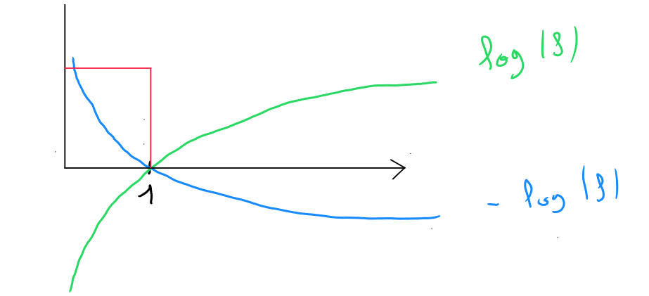
If we zoom in on this section and assume $y = 1$ for the loss function $L(f_{\vec{w},b}(\vec{x}^{(i)}), y^{(i)})$ and our model predicts :

• If the model predicts $1$, the loss is $0$ ;
• If the model predicts $0.5$, the loss is $-\ln(0.5) \approx 0.69$ ( natural logarithm ) ;
• If the model predicts $0.2$, the loss is $-\ln(0.2) \approx 1.61$ ;

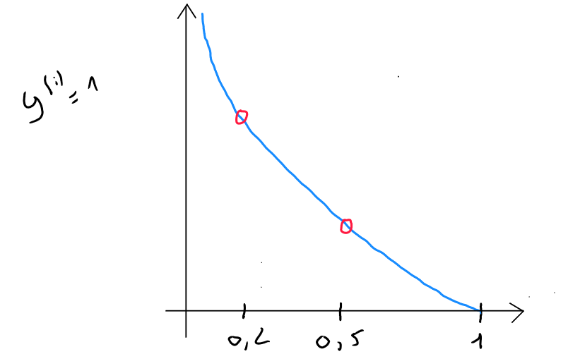
What we observe is that the algorithm will aim to reduce the loss and be as accurate as possible because predictions where $\hat{y} = 0$ but $y = 1$ result in significant loss.

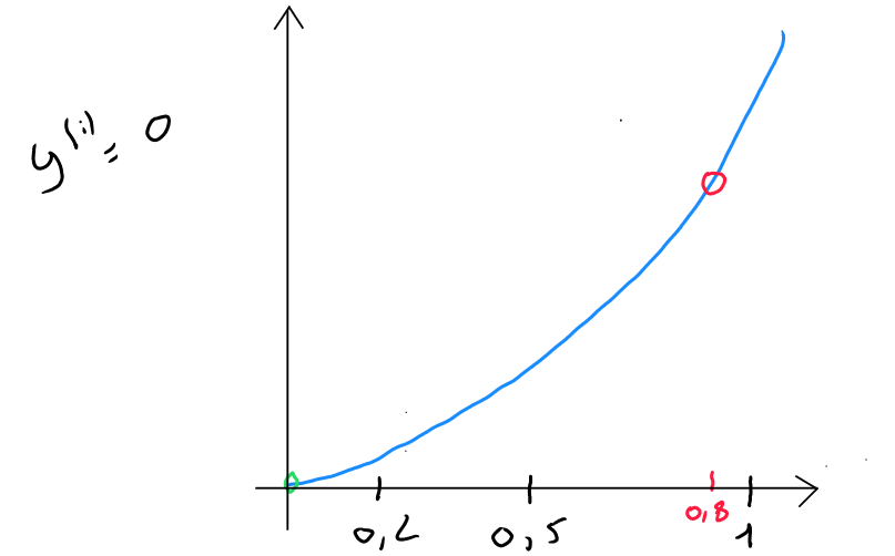
In the second case ($y = 0$), the algorithm will also aim to reduce the loss, and predictions where $\hat{y} = 1$ but $y = 0$ result in significant loss.

Therefore, transforming the cost function :

$$\textcolor{blue}{ L(f_{\vec{w},b}(\vec{x}^{(i)}), y^{(i)})}$$
$$L(f_{\vec{w},b}(\vec{x}^{(i)}),y^{(i)}) = \begin{cases} -log(f_{\vec{w},b}(\vec{x}^{(i)})) & \text{if } y^{(i)} = 1 \\ -log(1 - f_{\vec{w},b}(\vec{x}^{(i)})) & \text{if } y^{(i)} = 0 \end{cases}$$

Allows us to obtain a convex form and use gradient descent to find the local optimum.

Of course, the cost function applies to the entire dataset and will correspond to the sum of losses divided by $m$ :

$$J(\vec{w}, b) = \frac{1}{m} \sum_{i=1}^m L(f_{\vec{w},b}(\vec{x}^{(i)}),y^{(i)})$$

The gradient descent algorithm will therefore try to find the parameters $w, b$ that minimize the cost function.

The loss function :

$$L(f_{\vec{w},b}(\vec{x}^{(i)}),y^{(i)}) = \begin{cases} -log(f_{\vec{w},b}(\vec{x}^{(i)})) & \text{if } y^{(i)} = 1 \\ -log(1 - f_{\vec{w},b}(\vec{x}^{(i)})) & \text{if } y^{(i)} = 0 \end{cases}$$

Can be simplified as follows :

$$L(f_{\vec{w},b}(\vec{x}^{(i)}),y^{(i)}) = -y^{(i)}log(f_{\vec{w},b}(\vec{x}^{(i)}))- (1-y^{(i)})log(1-f_{\vec{w},b}(\vec{x}^{(i)}))$$

It is simplified because it combines both cases ($y=1$ or $y=0$) and automatically cancels one case if the other is assumed.

If $y^{(i)} = 1$ and we substitute the values of $y$ into the formula :

$$L(f_{\vec{w},b}(\vec{x}^{(i)}),y^{(i)}) = -\textcolor{blue}{y^{(i)}}log(f_{\vec{w},b}(\vec{x}^{(i)})) - (1-\textcolor{blue}{y^{(i)}})log(1-f_{\vec{w},b}(\vec{x}^{(i)}))$$
$$L(f_{\vec{w},b}(\vec{x}^{(i)}),y^{(i)}) = -\textcolor{blue}{1}log(f_{\vec{w},b}(\vec{x}^{(i)})) - (1-\textcolor{blue}{1})log(1-f_{\vec{w},b}(\vec{x}^{(i)}))$$

The right-hand side is canceled because $(1-1)*log... = 0*log... = 0$, and thus :

$$L(f_{\vec{w},b}(\vec{x}^{(i)}),y^{(i)}) = \textcolor{blue}{-y^{(i)}log(f_{\vec{w},b}(\vec{x}^{(i)}))}\textcolor{red}{ - (1-y^{(i)})log(1-f_{\vec{w},b}(\vec{x}^{(i)}))}$$

As a result, we get :

$$\textcolor{blue}{-1log(f_{\vec{w},b}(\vec{x}^{(i)}))}$$

If $y^{(i)} = 0$ and we substitute the values of $y$ into the formula:

$$L(f_{\vec{w},b}(\vec{x}^{(i)}),y^{(i)}) = -\textcolor{blue}{y^{(i)}}log(f_{\vec{w},b}(\vec{x}^{(i)})) - (1-\textcolor{blue}{y^{(i)}})log(1-f_{\vec{w},b}(\vec{x}^{(i)}))$$
$$L(f_{\vec{w},b}(\vec{x}^{(i)}),y^{(i)}) = -\textcolor{blue}{0}log(f_{\vec{w},b}(\vec{x}^{(i)})) - (1-\textcolor{blue}{0})log(1-f_{\vec{w},b}(\vec{x}^{(i)}))$$

The left-hand side is canceled because $-0*log... = 0*log... = 0$, and thus :

$$L(f_{\vec{w},b}(\vec{x}^{(i)}),y^{(i)}) = \textcolor{red}{-y^{(i)}log(f_{\vec{w},b}(\vec{x}^{(i)}))}\textcolor{blue}{ - (1-y^{(i)})log(1-f_{\vec{w},b}(\vec{x}^{(i)}))}$$

As a result, we get :

$$\textcolor{blue}{-log(1 - f_{\vec{w},b}(\vec{x}^{(i)}))}$$

Let’s remember that the loss function is a part of the cost function (in blue) :

$$J(\vec{w}, b) = \frac{1}{m} \sum_{i=1}^m \textcolor{blue}{\frac{1}{2}((\vec{w} \cdot \vec{x}^{(i)} + b) - y^{(i)})^2}$$

Corrected Cost Function (Convex)

Therefore, if we want to rewrite the entire cost function, small transformations will be applied to the operators, and we will obtain the following final formula :

$$J(\vec{w}, b) = -\frac{1}{m} \sum_{i=1}^m \left[ y^{(i)}log(f_{\vec{w},b}(\vec{x}^{(i)})) + (1-y^{(i)})log(1-f_{\vec{w},b}(\vec{x}^{(i)})) \right]$$

This final cost function is derived from the principle of maximum likelihood estimation, which, in the context of logistic regression, allows for finding the parameters $w$ and $b$ in a convex form.

Corrected Cost Function (Convex) in Python

def compute_cost(X, y, w, b, lambda_= 1):

    m, n = X.shape
    
    cost = 0.
                                              
    for i in range(m):
        z = np.dot(X[i],w)+b
        f_wb = sigmoid(z)
        cost += -y[i]*np.log(f_wb) - (1-y[i])*np.log(1-f_wb)
    total_cost = cost/m
    reg_cost = (lambda_ / (2 * m)) * np.sum(np.square(w))
    total_cost += reg_cost

    return total_cost

Gradient Descent

Just like the gradient descent algorithm in linear regression, the goal of gradient descent in logistic regression is to find the model that minimizes the cost function $J(\vec{w}, b)$. Defining the values of $w$ and $b$ will allow us to define the probability of $y$ belonging to class 1 ( where class 1 is generally the negative class ) for each new value of $x$. $P(y = 1 | \vec{X}; \vec{w}, b)$.

$$f(z) = \frac{1}{1 + e^{(-(\vec{w} \cdot \vec{x} + b))}}$$

The full cost function :

$$J(\vec{w}, b) = -\frac{1}{m} \sum_{i=1}^m \left[ y^{(i)}log(f_{\vec{w},b}(\vec{x}^{(i)})) + (1-y^{(i)})log(1-f_{\vec{w},b}(\vec{x}^{(i)})) \right]$$

The implementation of the gradient to minimize the cost follows the same process as linear regression, namely :

For each iteration $(i)$, it is important to define, temporarily, the new value of $w$ and the new value of $b$ and then replace them simultaneously.

1. $temp_w = w_j - \alpha \frac{d}{dw} J(w, b) = w_j - \alpha \frac{1}{m} \sum_{i=1}^{m} [f_{w,b}(x^{(i)}) - y^{(i)}] x^{(i)}$ ;
2. $temp_b = b - \alpha \frac{d}{db} J(w, b) = b - \alpha \frac{1}{m} \sum_{i=1}^{m} [f_{w,b}(x^{(i)}) - y^{(i)}]$ ;
3. $w = temp_w$ ;
4. $b = temp_b$ ;

This definition of the gradient descent steps is entirely similar to linear regression. That’s normal ; what changes is how the model is defined afterward :

1. In linear regression, we have : $f_{\vec{w}, b}(\vec{x}) = \vec{w} \cdot \vec{x} + b$ ;
2. In logistic regression, we apply $f(z)$, which gives : $f(z) = \frac{1}{1 + e^{(-(\vec{w} \cdot \vec{x} + b))}}$ ;

warning

Even though the gradient descent algorithm appears similar for both linear and logistic regression, they are indeed two different algorithms because of how they are applied in the model.

Odds Ratio

In statistics, the Odds Ratio is a measure that quantifies the strength of association between an explanatory variable ( predictor ) and the probability of occurrence of the event we want to predict (class 1, often representing the negative aspect, e.g. Spam 1, Non-Spam 0; Sick 1, Healthy 0).

The odds ratio evaluates the change in the probability of $y = 1$ based on a one-unit increase in the explanatory variable.

Imagine we have 10 patients. Among them, 6 are sick and 4 have a fever. Among those with a fever, 3 are sick and 1 is not. The odds ratio will allow us to calculate the chance of having a fever when sick compared to not being sick and having a fever.

	Fever (p)	No Fever (q)	Total
Sick	3 (p)	3	6
Not Sick	1 (q)	3	4
Total	4	6	10

To calculate the odds ratio, we use the following formula (where $p$ is the proportion of sick patients with a fever, and $q$ is the proportion of non-sick patients with a fever) :

$$OR = \frac{\frac{p}{(1 - p)}}{\frac{q}{(1 - q)}} = \frac{p(1 - q)}{q(1 - p)}$$

In our example: $p = 3/6$ which equals $0.5$; $q = 1/4$ which equals $0.25$.

Thus :

$$\frac{\frac{0.5}{(1 - 0.5)}}{\frac{0.25}{(1 - 0.25)}} = \frac{0.5(1 - 0.25)}{0.25(1 - 0.5)} = \frac{0.375}{0.125} = 3$$

The result indicates that the odds of having a fever are 3 times higher for sick patients than for non-sick patients ( the probabilities are 0.5 versus 0.25 ).

warning

This does not indicate the probability of having a fever if you're sick or being sick if you have a fever! It's simply the association between sickness and fever.

In logistic regression, the odds ratio is calculated from the coefficient $w$ found by the gradient descent method. The odds ratio for an explanatory variable is given by $e^{w}$. For example, if the gradient descent identifies a $w$ value of $0.03$ for fever, the odds ratio is $e^{0.03} = 1.03$. This means the chances of being sick increase by $3\%$ when a patient has a fever compared to one who does not.

However, the odds ratio does not calculate probability but helps to better understand the multiplicative factor of chance that the event decreases or increases as the explanatory variable increases by one unit. It allows for easier comparison of the impact of different explanatory variables on the probability of the event.

The odds ratio helps in understanding the model’s functioning and results.

As a reminder, the probability will be calculated based on the $x$ value of a new record and the $b$ and $w$ values identified by the gradient descent.

Gradient Descent in Python:

def compute_gradient(X, y, w, b, lambda_=1):

    m, n = X.shape
    dj_dw = np.zeros(w.shape)
    dj_db = 0.

    for i in range(m):
        f_wb_i = sigmoid(np.dot(X[i],w) + b)          
        err_i  = f_wb_i  - y[i]                      
        for j in range(n):
            dj_dw[j] = dj_dw[j] + err_i * X[i,j]     
        dj_db = dj_db + err_i
    dj_dw = dj_dw/m                                  
    dj_db = dj_db/m                                  
    dj_dw += (lambda_ / m) * w
    return dj_db, dj_dw

Launching Gradient Descent:

def gradient_descent(X, y, w_in, b_in, cost_function, gradient_function, alpha, num_iters, lambda_):


    m = len(X)

    J_history = []
    w_history = []

    for i in range(num_iters):

        dj_db, dj_dw = gradient_function(X, y, w_in, b_in, lambda_)

        w_in = w_in - alpha * dj_dw
        b_in = b_in - alpha * dj_db
        
        if i<100000:      
            J_history.append( cost_function(X, y, w_in, b_in, lambda_))
        
        if i > 1 and abs(J_history[-1] - J_history[-2]) < 0.000001:
            print(f"Early stopping at iteration {i} as cost change is less than 0.000001")
            break 
            
        if i% math.ceil(num_iters / 10) == 0:
            print(f"Iteration {i:4}: Cost {J_history[-1]} ",
                  f"dj_dw: {dj_dw}, dj_db: {dj_db}  ",
                  f"w_in: {w_in}, b_in:{b_in}")

    return w_in, b_in, J_history, w_history 


np.random.seed(1)
initial_w = np.zeros(x_train.shape[1])  
initial_b = 0

lambda_=0.01
iterations = 1000
alpha = 0.003

w,b, J_history,_ = gradient_descent(x_train ,y_train, initial_w, initial_b,
                                   compute_cost, compute_gradient, alpha, iterations, lambda_)

$$f(z) = \frac{1}{1 + e^{(-(\vec{w} \cdot \vec{x} + b))}}$$

Regularization

The principle of regularization in logistic regression is identical to what we find in linear regression.

That means, in the case of underfitting, the main option is to add more variables or additional records, and in overfitting, we also find basic options like increasing or reducing variables ( Variable Selection ) and increasing the number of records.

As with linear regression, reducing the number of variables is applied via the concept of feature engineering or through specific techniques.

If, for specific reasons, we as data scientists must keep all variables, we can also counter overfitting by applying regularization to logistic regression.

Recall that the concept of regularization involves reducing the impact of certain variables by assigning them a lower weight. Specifically, the idea is to make the learning algorithm reduce the values of parameters without forcing them to be set to $0$. Regularization primarily applies to the values of $w$, although regularization could also be applied to the parameter $b$.

This penalty is applied by adding the following regularization term to the modified cost function of logistic regression :

$$J(\vec{w}, b) = -\frac{1}{m} \sum_{i=1}^m \left[ y^{(i)}log(f_{\vec{w},b}(\vec{x}^{(i)})) + (1-y^{(i)})log(1-f_{\vec{w},b}(\vec{x}^{(i)})) \right] + \textcolor{blue}{\frac{\lambda}{2m} \sum_{j=1}^n w_j^2}$$

tip

Regularized Gradient Descent

$J(\vec{w}, b) = -\frac{1}{m} \sum_{i=1}^m \left[ y^{(i)}log(f_{\vec{w},b}(\vec{x}^{(i)})) + (1-y^{(i)})log(1-f_{\vec{w},b}(\vec{x}^{(i)})) \right] + \textcolor{blue}{\frac{\lambda}{2m} \sum_{j=1}^n w_j^2}$

1. $temp_w = w - \alpha \frac{d}{dw} J(w, b) = w - \alpha \left( \frac{1}{m} \sum_{i=1}^{m} [f_{w,b}(x^{(i)}) - y^{(i)}] x^{(i)} + \textcolor{blue}{\frac{\lambda}{m} w}\right)$ ;
2. $temp_b = b - \alpha \frac{d}{db} J(w, b) = b - \alpha \left( \frac{1}{m} \sum_{i=1}^{m} [f_{w,b}(x^{(i)}) - y^{(i)}]\right)$;
3. $w = temp_w$ ;
4. $b = temp_b$ ;

Complete Python Code

import numpy as np
import pandas as pd
from sklearn.preprocessing import StandardScaler
from sklearn.model_selection import train_test_split
import math, copy
from sklearn.metrics import confusion_matrix



data = pd.read_csv('data.csv')
data

x = data[['x_1', 'x_2', 'x_3', 'x_4', 'x_5', '...', 'x_n']].values  
y = data['y'].values  


scaler_x = StandardScaler()
scaler_y = StandardScaler()

x = scaler_x.fit_transform(x)

x_train, x_test, y_train, y_test = train_test_split(x, y, test_size=0.4, random_state=42)

#polynomial
"""
# Chargement des données
data = pd.read_csv('data.csv')

# Séparation des caractéristiques et de la cible
x = data[['x_1', 'x_2', 'x_3', 'x_4', 'x_5', '...', 'x_n']].values  
y = data['y'].values  

# Génération des termes polynomiaux de degré 3
poly = PolynomialFeatures(degree=3)
x_poly = poly.fit_transform(x)

# Standardisation des données polynomiales
scaler_x = StandardScaler()
x_poly = scaler_x.fit_transform(x_poly)
x_train, x_test, y_train, y_test = train_test_split(x, y, test_size=0.4, random_state=42)
"""
# /Polynomial

def sigmoid(z):

    g = 1/(1+np.exp(-z))


    return g


def compute_cost(X, y, w, b, lambda_= 1):

    m, n = X.shape
    
    cost = 0.
                                              
    for i in range(m):
        z = np.dot(X[i],w)+b
        f_wb = sigmoid(z)
        cost += -y[i]*np.log(f_wb) - (1-y[i])*np.log(1-f_wb)
    total_cost = cost/m

    reg_cost = (lambda_ / (2 * m)) * np.sum(np.square(w))
    total_cost += reg_cost

    return total_cost

def compute_gradient(X, y, w, b, lambda_=1):

    m, n = X.shape
    dj_dw = np.zeros(w.shape)
    dj_db = 0.

    for i in range(m):
        f_wb_i = sigmoid(np.dot(X[i],w) + b)          
        err_i  = f_wb_i  - y[i]                      
        for j in range(n):
            dj_dw[j] = dj_dw[j] + err_i * X[i,j]     
        dj_db = dj_db + err_i
    dj_dw = dj_dw/m                                  
    dj_db = dj_db/m                                  
    dj_dw += (lambda_ / m) * w
    return dj_db, dj_dw


def gradient_descent(X, y, w_in, b_in, cost_function, gradient_function, alpha, num_iters, lambda_):


    m = len(X)

    J_history = []
    w_history = []

    for i in range(num_iters):

        dj_db, dj_dw = gradient_function(X, y, w_in, b_in, lambda_)

        w_in = w_in - alpha * dj_dw
        b_in = b_in - alpha * dj_db
        
        if i<100000:      
            J_history.append( cost_function(X, y, w_in, b_in, lambda_))
        
        if i > 1 and abs(J_history[-1] - J_history[-2]) < 0.000001:
            print(f"Early stopping at iteration {i} as cost change is less than 0.000001")
            break 
            
        if i% math.ceil(num_iters / 10) == 0:
            print(f"Iteration {i:4}: Cost {J_history[-1]} ",
                  f"dj_dw: {dj_dw}, dj_db: {dj_db}  ",
                  f"w_in: {w_in}, b_in:{b_in}")

    return w_in, b_in, J_history, w_history 


np.random.seed(1)
initial_w = np.zeros(x_train.shape[1])  
initial_b = 0

lambda_=0.01
iterations = 1000
alpha = 0.003

w,b, J_history,_ = gradient_descent(x_train ,y_train, initial_w, initial_b,
                                   compute_cost, compute_gradient, alpha, iterations, lambda_)

def predict(X, w, b):

    m, n = X.shape
    p = np.zeros(m)

    for i in range(m):
        z_wb = np.dot(X[i],w)
        
        for j in range(n):
            
            z_wb += 0

        z_wb += b

        f_wb = sigmoid(z_wb)

        p[i] =  1 if f_wb>=0.5 else 0

    return p


p = predict(x_test, w, b) 
confusion = confusion_matrix(y_test, p)


TP = confusion[1, 1]  # True positive
FP = confusion[0, 1]  # False positive
TN = confusion[0, 0]  # True negative
FN = confusion[1, 0]  # False negative

print("Confusion matrix :")
print(confusion)
print("True positive (TP):", TP)
print("False positive (FP):", FP)
print("True negative (TN):", TN)
print("False negative (FN):", FN)