Clustering

Automatic classification, also known as segmentation or clustering, is the most widespread technique in unsupervised learning.

It is used when we have a large volume of data in which we seek to distinguish homogeneous subsets, susceptible to differentiated treatments and analyses.

Therefore, it is an unsupervised technique often used as a preliminary step ( pre-processing ) before applying a supervised technique to improve prediction performance.

As a reminder, there are two types of learning : supervised and unsupervised. Until now, we have dealt with supervised techniques, meaning techniques from which we make predictions ( classification or estimation ).

warning

Although the term « classement » in French is translated as « classification » in English and refers to a supervised technique, the term « classification » in French is translated as « clustering » in English.

• Clustering (EN) − Classification (FR) : dividing the entire dataset into relatively homogeneous subgroups, maximizing the similarity of records within the group and minimizing the similarity outside the group.
• Classification (EN) – Classement (FR) : assigning each record to a class, among several predefined classes, based on the characteristics of the record described as explanatory variables ( predictors ). The result allows each individual to be assigned to the best class.

Since we are addressing unsupervised techniques, it is important to recall a fundamental difference from supervised learning : in unsupervised learning, there are only $x$ ; no $y$, and all records are used - there is no partition for a training phase -. The technique is applied to the entire dataset, and we, as data scientists, must interpret the result.

However, there is a connection between these two families : most predictive algorithms struggle with too many variables due to correlations between them, which hinder their predictive power. Clustering allows the formation of homogeneous groups that can be described by a small number of variables specific to each group. Moreover, sometimes it is useful for a predictive algorithm to handle missing values without substituting them with a priori values like the average of the records. One solution is to apply a clustering technique beforehand to group individuals with missing values into clusters and then impute the average of those groups to replace the missing value.

Thus, we want to segment a heterogeneous population into homogeneous subgroups or clusters. The qualities of a cluster are :

• strong intra-class similarity
• low inter-class similarity

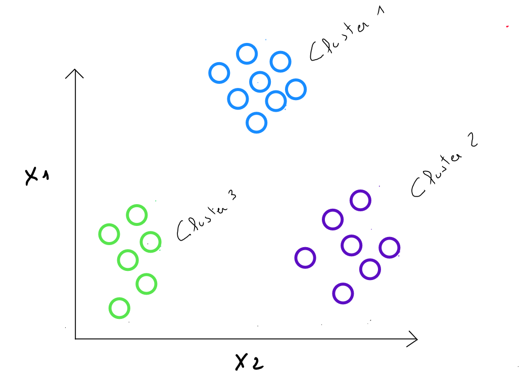
K-means

The K-means method is one of the main partitioning methods, aimed at partitioning individuals for whom we have measurements into different classes.

We seek to group individuals that are as similar as possible ( from the point of view of the measurements we have ) while separating the classes as much as possible from one another.

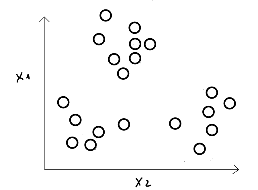
Steps

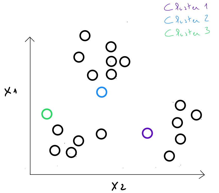
Step 1 : we choose $k$ individuals as initial class centers ( we define the number of classes and the individuals considered as the centers of these classes randomly ) - in reality, we will see later that the algorithm « tests » many configurations to identify the best possible distribution of the data -.

Example $k = 3$

Step 2 : we calculate the distances between each individual and each center from the previous step. We assign each individual to the closest center, which defines $k$ classes.

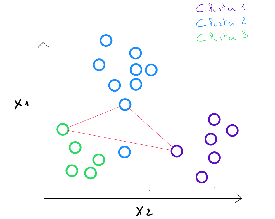
Step 3 : We replace the initial class centers with the barycenters of the $k$ classes. The new centroids are calculated by taking the average of the coordinates of all the points belonging to each cluster. ( These barycenters are not necessarily existing data points ).

For example, in cluster 2 identified in step $2$, if we obtain the values $4,6$ and $8$ for this cluster, in step 3, the new center will be $\frac{4 + 6 + 8}{3}$, which equals $6$.

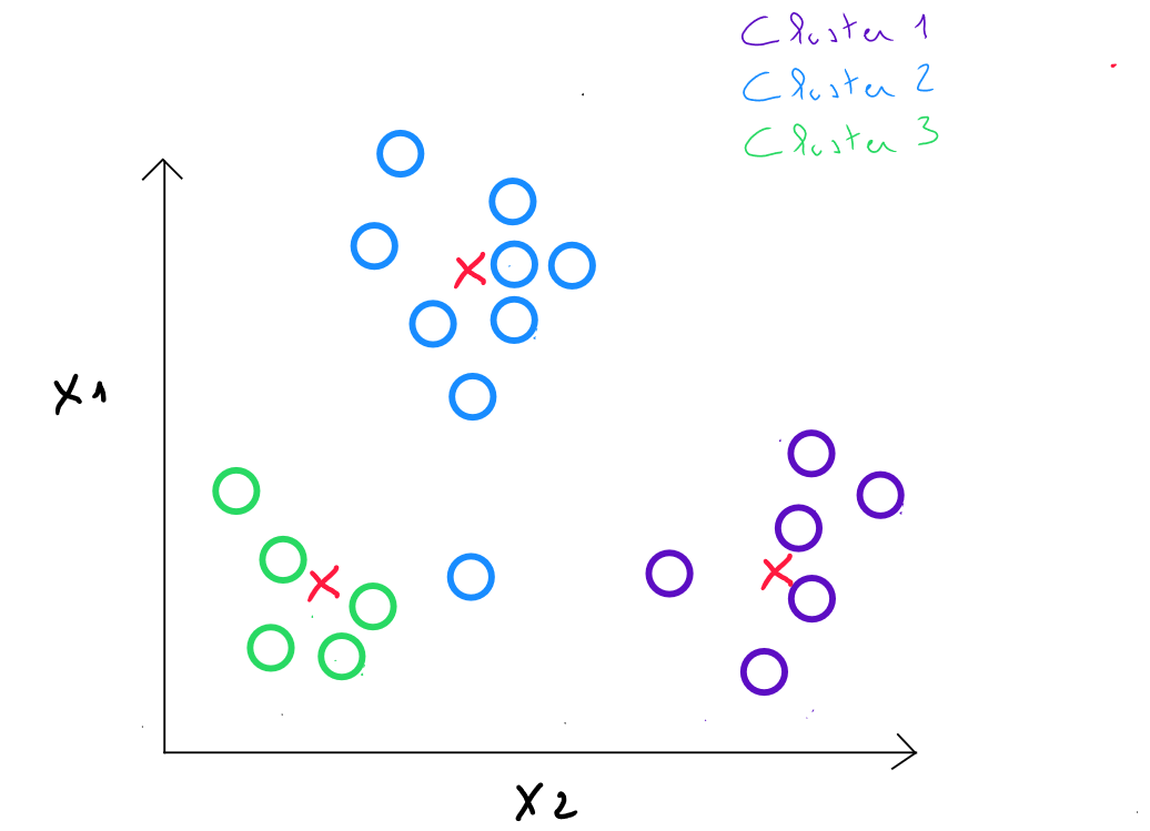
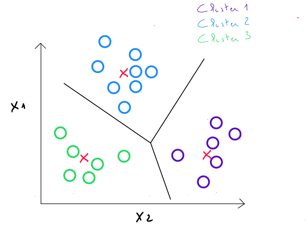
Step 4: we calculate the distances between each individual and each center, and we assign each individual to the closest center.

Steps 3 and 4 are repeated in iterations until the centers remain stable enough ( comparing their displacement to the distances between the initial centers ).

Distance Calculation

Distances can be defined in several ways, but generally, the following properties are required :

• a distance is non-negative : $d_{ij} >=0$
• self-proximity principle : $d_{ii} = 0$ (the distance of a record from itself is 0)
• Symmetry principle : $d_{ij} = d_{ji}$
• triangle inequality principle : $d_{ij} <= d_{ik} + d_{kj}$ ( the distance between any pair cannot exceed the sum of the distances between two other pairs )

As in the K-NN Nearest Neighbors technique, the concept of distance between two records ( proximity – similarity ) is calculated based on quantitative variables. Therefore, it is important in some cases to transform the data to be able to apply distance calculations. If the variables are ordinal qualitative, they must be numerized. If the variables are nominal qualitative, we must perform one-hot encoding.

The three most commonly used distances are Euclidean distance, Manhattan distance, and Minkowski distance.

Euclidean Distance

Euclidean distance is the most commonly used method for calculating the distance between two records because it is considered the least computationally intensive. It is simply the shortest distance between point A and point B.

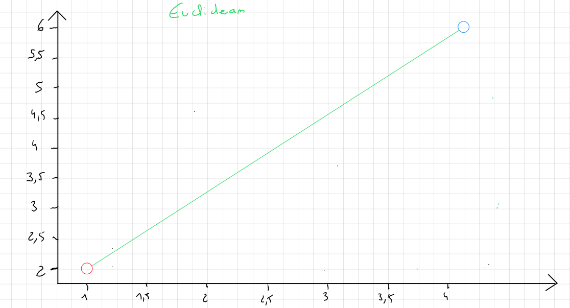
The formula for Euclidean distance is :

$$d(p, q) = \sqrt{\sum_{i=1}^{n} (p_i - q_i)^2}$$

or

$$d(p, q) = \sqrt{(p_{i1} - q_{i1})^2 + (p_{i2} - q_{i2})^2 + \dots + (p_{in} - q_{in})^2}$$

For the following example :

ID	$x_1$	$x_2$
01	2.04	3.2
02	1.98	3.8

The distance is calculated as follows :

$$d_{1,2} = \sqrt{(2.04 - 1.98)^2 + (3.2 - 3.8)^2} = 0.603$$

The distance is calculated for all records $d_{1,3}, d_{1,4}, d_{1,...}, d_{1,n}$.

Euclidean distance is heavily influenced by the scale of each variable. Therefore, it is common practice to normalize the data to convert them to the same scale. Moreover, it does not account for possible relationships between variables ( correlation ) and is sensitive to outliers.

Manhattan Distance

If the data contain outliers and, for specific reasons, these outliers are not removed, we favor the Manhattan distance, which focuses on the absolute value of the differences rather than the square of the differences.

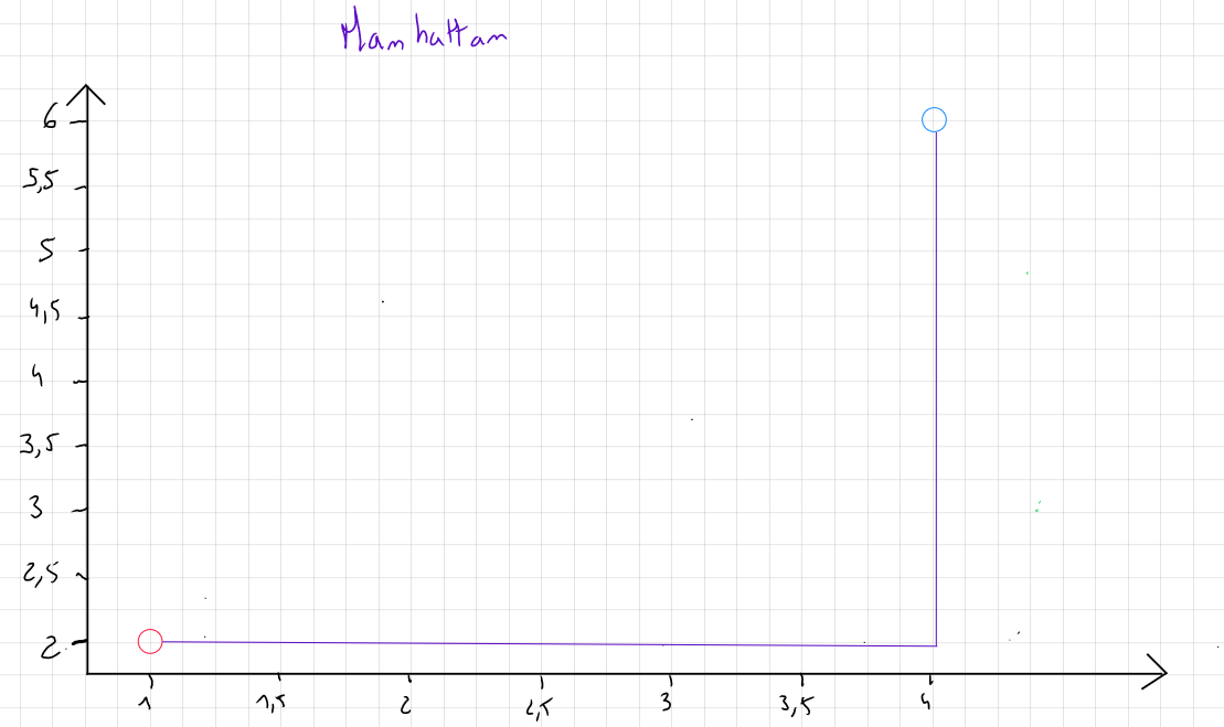
This measure is named after the city of Manhattan because, in two dimensions, it represents the distance a taxi would travel in a city where streets are either parallel or perpendicular to one another.

The formula for Manhattan distance is :

$$d(p, q) = \sum_{i=1}^{n} |p_i - q_i|$$

or

$$d(p, q) = |p_{i1} - q_{i1}| + |p_{i2} - q_{i2}| + \dots + |p_{in} - q_{in}|$$

For the following example :

ID	$x_1$	$x_2$
01	2.04	3.2
02	1.98	3.8

The distance is calculated as follows :

$$d_{1,2} = |2.04 - 1.98| + |3.2 - 3.8| = 0.66$$

The distance is calculated for all records $d_{1,3}, d_{1,4}, d_{1,...}, d_{1,n}$.

Minkowski Distance

Minkowski distance generalizes Euclidean and Manhattan distances.

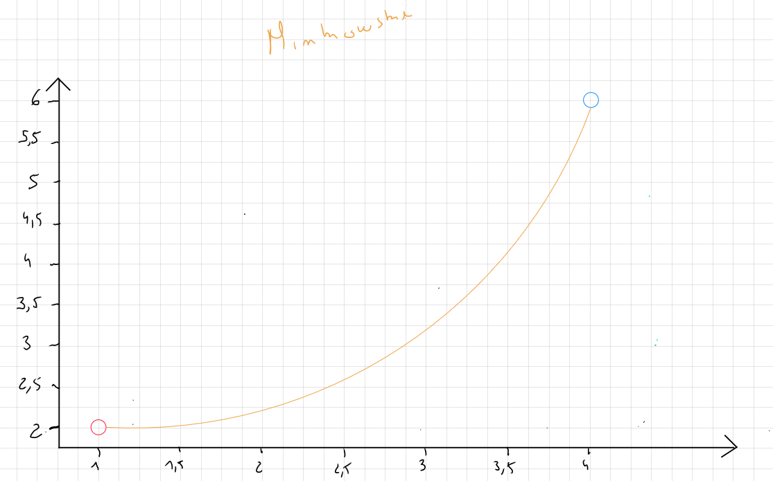
The formula for Minkowski distance is :

$$d(p, q) = \left( \sum_{i=1}^{n} |p_i - q_i|^p \right)^{\frac{1}{p}}$$

or

$$d(p, q) = (|p_{i1} - q_{i1}|^p + |p_{i2} - q_{i2}|^p + \dots + |p_{in} - q_{in}|^p)^\frac{1}{p}$$

where $p$ is a power parameter that controls how the differences between the coordinates of the points are aggregated. This parameter can take several values, but in practice, $p = 1$ corresponds to the Manhattan distance, $p = 2$ corresponds to the Euclidean distance, and values of $p > 2$ are more sensitive to large differences between values.

In practice, Minkowski distance allows testing multiple combinations by modifying the value of $p$ according to the analyst's needs.

For the following example :

ID	$x_1$	$x_2$
01	2.04	3.2
02	1.98	3.8

The distance is calculated as follows :

$$d_{1,2} = (|2.04 - 1.98|^3 + |3.2 - 3.8|^3)^\frac{1}{3} = 0.600$$

The distance is calculated for all records $d_{1,3}, d_{1,4}, d_{1,...}, d_{1,n}$.

Algorithm

Random initialization of $k$ cluster centroids $𝜇_1,𝜇_2,…,𝜇_𝑘$.
Repeat $[$

1. assign points to cluster centroids
For $𝑖 =1$ to $𝑚$:

$𝑐^{(𝑖)}=$ index (from $1$ to $k$) of the closest cluster centroid.




2. move the clusters
For $𝑘=1$ to $𝑘$:


$𝜇_𝑘=$mean of the points assigned to cluster $𝑘$.
$𝜇_1= \frac{1}{5}*[𝑥^1+𝑥^4+𝑥^7+𝑥^9+𝑥^3]$.


$]$

Initialization of $k$

The initialization of the cluster centers and the number of clusters is a delicate element because the arbitrary choice of $k$ ( number of clusters ) and their random initialization can result in different clusters. This is why, when we select $k$ ( for example, $k = 3$ ), we iterate over different initializations of $k$ among the data and select the model with the smallest cost function.

This means that (1) : the algorithm will iterate over different values of $k$ to identify the best way to group the data, and for each value of $k$, the algorithm will iterate over different initializations of $k$.

A general rule is to loop ( depending on the number of examples ) over 1 to 100 different initializations for each choice of $k$ (e.g. $k = 3$), but it can increase to 50 to 1000 to get a better score.

Cost Function

We can thus identify a cost function that seeks to minimize the intra-cluster variance ( intra-class ), i.e. select data grouping results where the data are closest to each other. Specifically, this cost function is calculated for several values of $k$. For each value of $k$, it will iterate over the number of clusters, and for each cluster, several centroid initialization values will be tested.

For example, for $k = 3$, the algorithm will run 1 to 100 initializations for cluster 1, cluster 2, and cluster 3. It will select the initialization that minimizes the intra-cluster variance ( intra-class ).

$𝐽(𝑐^{(1)},…, 𝑐^{(𝑚)},𝜇_1,…,𝜇_𝑘)= \frac{1}{m}\sum_{i=1}^{m} \left\| x^{(i)} - \mu_{c^{(i)}} \right\|^2$

Thus, the cost function distributes the clusters by obtaining the lowest intra-class inertia.

Intra-Class Inertia

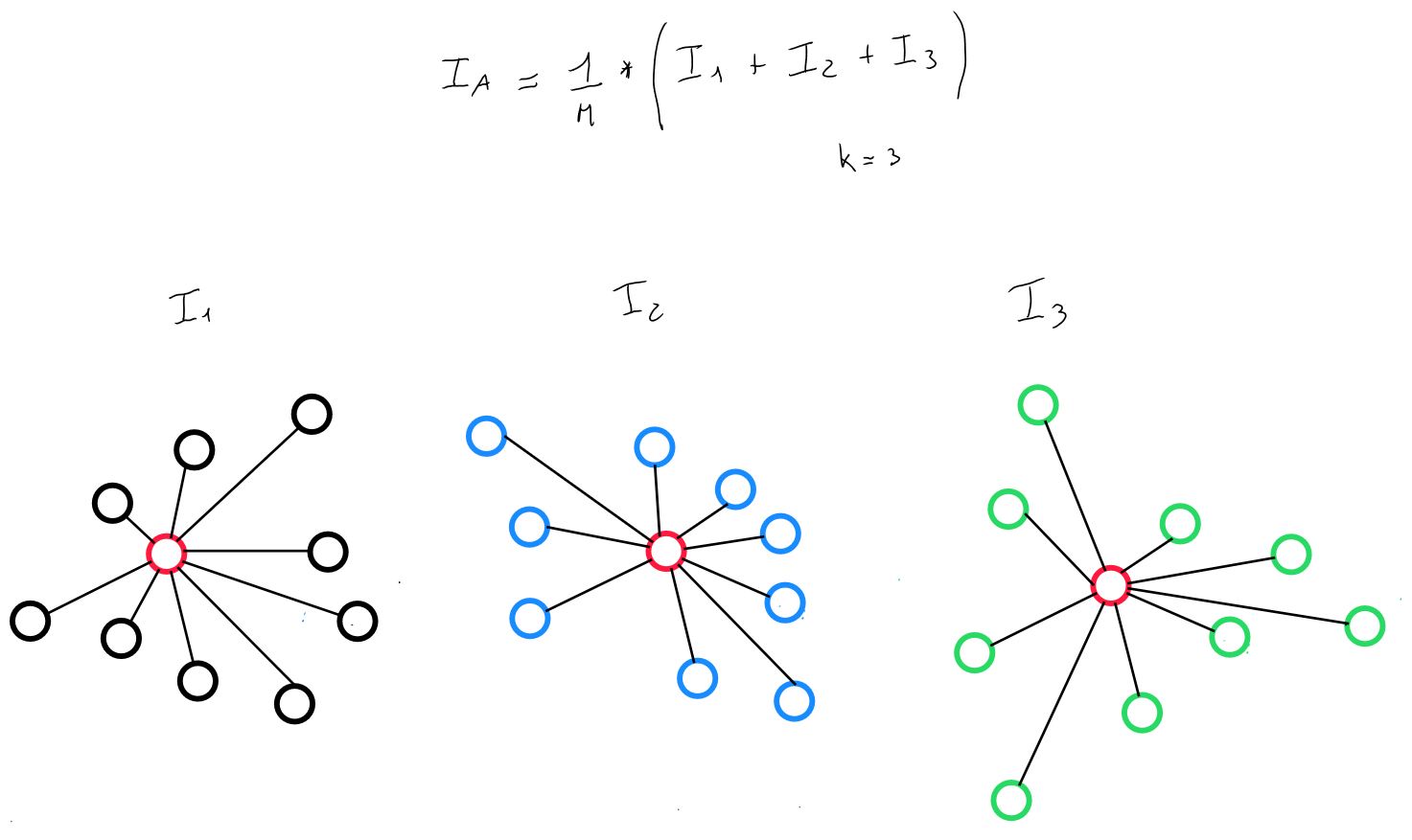
The inertia of a cluster ( class ) $I_k$ is calculated as follows, relative to its barycenter :

$$\sum_{i \in I} P_i (x_i - \overline{x_j})^2$$

If the population is segmented into $k$ clusters, with inertias $I_1,…,I_𝑘$, the intra-cluster inertia is, by definition, the sum of the total inertias of each cluster.

$$I_A = \frac{1}{m} \sum_{i=1}^{m} \left\| x^{(i)} - \mu_{c^{(i)}} \right\|^2 = J(c^{(1)}, \dots, c^{(m)}, \mu_1, \dots, \mu_k)$$

Selection of $k$

So far, we have seen how to minimize the cost function for clusters where the choice of $k$ was arbitrary ($k = 3$ ). However, the goal is to minimize the cost function for a clustering technique with $k$ clusters, without knowing the ideal number of clusters in advance for segmenting our data.

Again, the idea is to perform iterations :

• if $k = 2$, then $J(k)$ is calculated by performing random initialization iterations of $k$ ( for example, 1 to 1000 ), because the initial choice of $k$ values can impact the result.
for each random initialization of 2 values of $k$ ( since there are 2 clusters ), the algorithm calculates the cost function $I_A = \frac{1}{m} \sum_{i=1}^{m} \left\| x^{(i)} - \mu_{c^{(i)}} \right\|^2 = J(c^{(1)}, \dots, c^{(m)}, \mu_1, \dots, \mu_k)$ and selects the two initialization values that minimize the intra-cluster inertia for $k = 2$.
• if $k = 3$, the same process ( previous 2 steps ) is repeated, and the three initialization values that minimize the cost are selected.
for each random initialization of 3 values of $k$ ( since there are 3 clusters ), the algorithm calculates the cost function $I_A = \frac{1}{m} \sum_{i=1}^{m} \left\| x^{(i)} - \mu_{c^{(i)}} \right\|^2 = J(c^{(1)}, \dots, c^{(m)}, \mu_1, \dots, \mu_k)$ and selects the three initialization values that minimize the intra-cluster inertia for $k = 3$.
• the same process is carried out for different scenarios of $k$ (e.g., $k > 1$ and $<= 20$).
• for each scenario, the initialization values corresponding to $k$ are identified, and more importantly, a cost is determined, as it minimizes the intra-cluster inertia for the corresponding $k$.
• the choice of $k$ will consist of selecting, among the costs of each scenario of $k$ (e.g., $k = 2, k = 3, k = 4, ..., k = 20$), the scenario where the decrease in cost is the last significant drop when moving from $k$ to $k + 1$.

If we represent on the y-axis the cost function values and on the x-axis the $k$ values, we will obtain the following graph :

tip

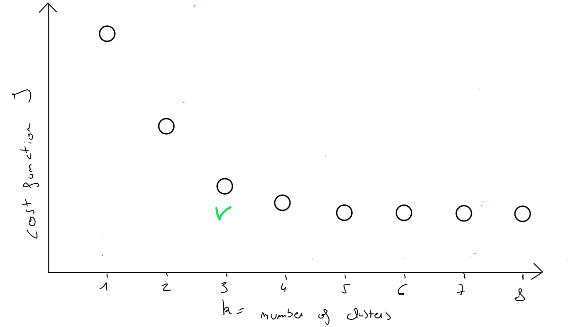
If the last significant decrease in $J$ occurs when going from $k$ to $k +1$ classes, then the partition into $k$ classes is good ! Selecting the smallest value of $J$ would be incorrect because if $k =$ number of records, then the cost would be $0$.

This selection of $k$ is called the elbow method ( because the best selection of the cost function and therefore of $k$ corresponds to the shape of an elbow ).

Hierarchical Ascending Classification

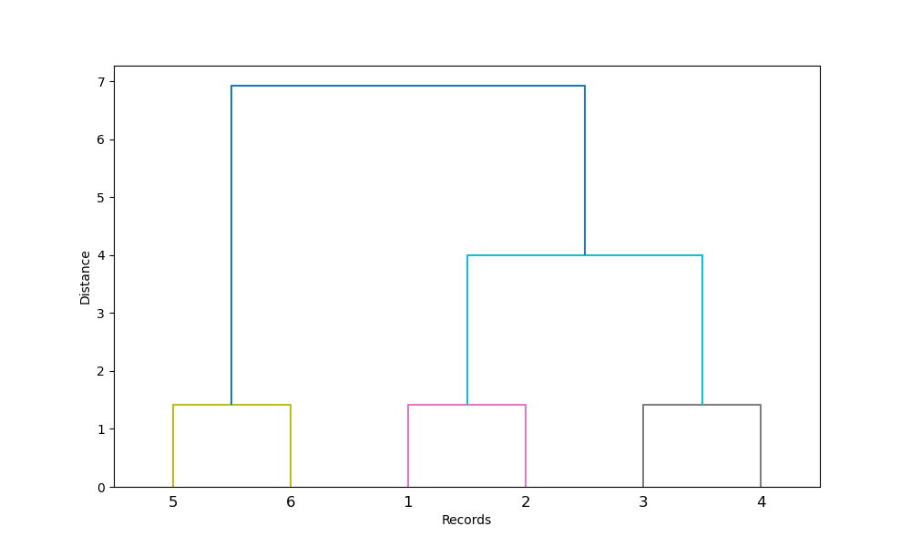
Hierarchical ascending classification is a technique from the clustering family, distinguished by the fact that it produces nested partitions with increasing heterogeneity, from the partition into $k$ classes where each object is isolated, to the partition into $k = 1$ class that groups all objects together.

This method is also carried out in several steps.

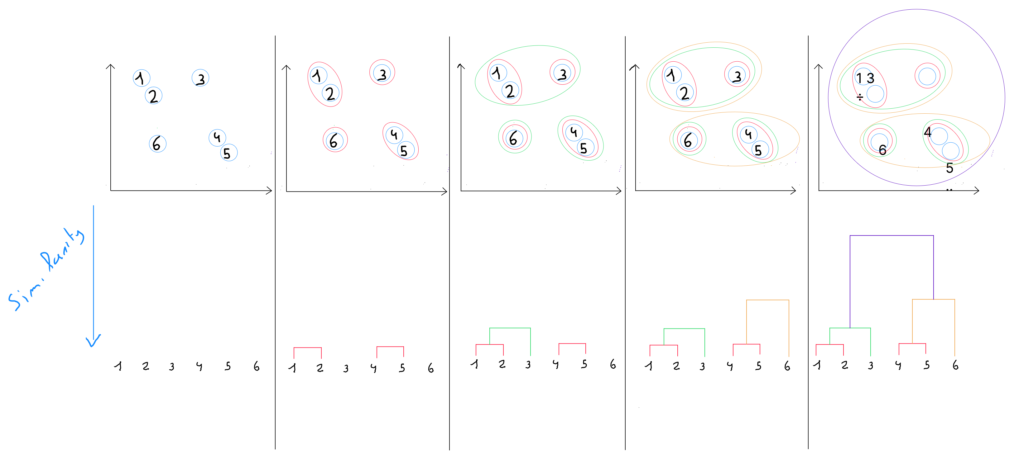
step 1 : the algorithm defines by default each record as an individual cluster. In other words, each individual is a class. If $n = 16$, we start with 16 clusters, each containing one record.

step 2 : the distances between the classes are calculated.

• in the first distance calculation, when $k = n$, Euclidean distance is generally used, or Manhattan or Minkowski.
• at the next hierarchical levels ( when a class has more than one element ), other calculation methods are used ( described below ).

step 3 : ( at a higher hierarchical level ), the closest classes are merged into a single class.

step 4 : The algorithm repeats Step 2 until obtaining a single class that contains all the records.

Dendrogram

The sequence of partitions is represented by a tree called a dendrogram. This tree can be cut at various heights to obtain more or fewer classes. It allows for the visualization of how the partitions are made, with the understanding that the closer to the base of the dendrogram, the stronger the similarity and the closer the distance.

Practically, we choose at which height to cut the dendrogram to select a certain number of classes. This choice can be arbitrary depending on the desired number of clusters, but it is recommended to select the height that optimizes intra-class similarity.

Inter-Class Distances

The hierarchical ascending classification algorithm works by searching at each step for the closest clusters to merge, and the « essence » of the algorithm lies in the definition of the distance between two classes ( clusters ) A and B.

This distance can be defined in multiple ways, with each method having advantages and disadvantages, and applying in very specific conditions ( class shapes ).

warning

Reminder : in Step 1, Euclidean distance is used to group the closest points.

Complete Linkage Method

The complete linkage method returns the maximum distance between two data points from two clusters :

maximum distance between points $i$ and $j$, where $i$ belongs to R and $j$ belongs to S.

$$L(R, S) = \max(D(i, j)), \quad i \in R, \, j \in S$$

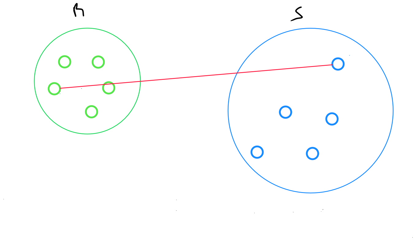
By definition, this measure is very sensitive to outliers, and as such, is rarely used.

Single Linkage Method

The single linkage method returns the minimum distance between two data points from two clusters :

minimum distance between points $i$ and $j$, where $i$ belongs to R and $j$ belongs to S.

$$L(R, S) = \min(D(i, j)), \quad i \in R, \, j \in S$$

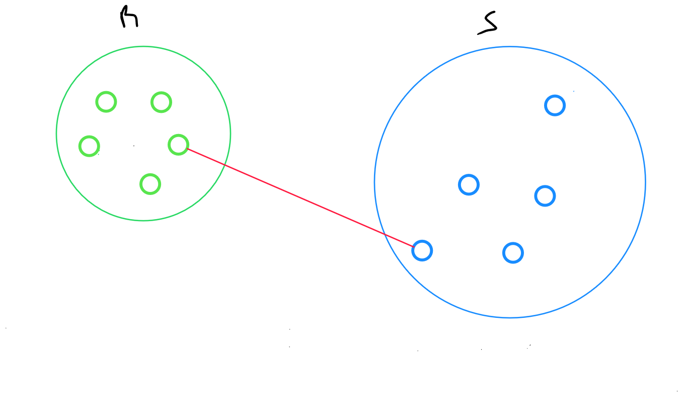
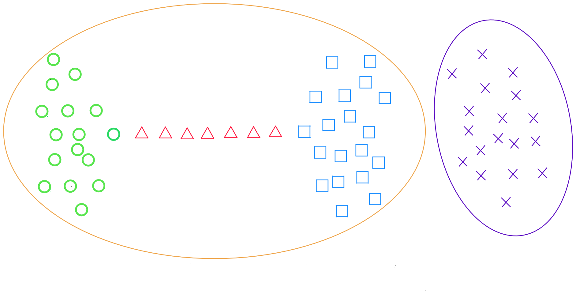
The main weakness of this method is its sensitivity to the « chain effect » : two distant classes connected by a chain of closely related individuals may end up being grouped together.

Average Linkage Method

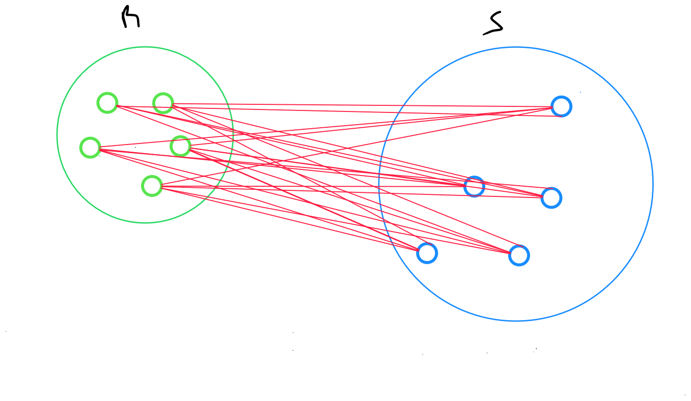
The average linkage method returns the average distance between all data points in two clusters :

for two clusters R and S, the distance between all records $i$ in R and all individuals $j$ in S is calculated, and then the arithmetic mean of these distances is defined.

$$L(R, S) = \frac{1}{n_R n_S} \sum_{i=1}^{n_R} \sum_{j=1}^{n_S} D(i, j), \quad i \in R, \, j \in S$$

where

$$n_R \text{ is the number of points in } R$$$$n_S \text{ is the number of points in } S$$

Centroid Method

The centroid method returns the distance between the centroids of two clusters :

for two clusters R and S, the distance between the centroid $u_i$ of R and the centroid $u_j$ of S is calculated.

$$L(R, S) = \|\mathbf{c}_R - \mathbf{c}_S\|$$

where

$$\mathbf{c}_R = \frac{1}{n_R} \sum_{i \in R} \mathbf{x}_i$$

and

$$\mathbf{c}_S = \frac{1}{n_S} \sum_{j \in S} \mathbf{x}_j$$

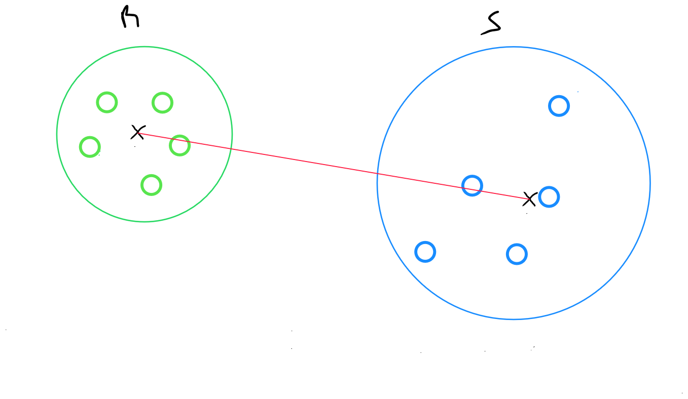
This is the simplest method to calculate and is more robust to outliers, but it is less precise.

Ward’s Method

Ward’s method best aligns with the goal of hierarchical ascending classification, which is to achieve high inter-class inertia.

For transitioning from a classification with $k+1$ classes to one with $k$ classes ( merging classes at a higher hierarchical level ), the goal is to merge the two classes that will least reduce inter-class inertia. The distance between two classes is the square of the distance between their centroids, weighted by the sizes of the two clusters. Ward’s distance is sensitive to outliers but is the most commonly used.

$$D_{KL} = \frac{\|\mathbf{\bar{x}}_K - \mathbf{\bar{x}}_L\|^2}{\frac{1}{N_K} + \frac{1}{N_L}}$$

Code Python K-Means

import os
os.environ["OMP_NUM_THREADS"] = "2"

import numpy as np
import pandas as pd
from sklearn.datasets import make_blobs
from sklearn.preprocessing import MinMaxScaler
from sklearn.cluster import KMeans
import matplotlib.pyplot as plt

'''
##Synthetic dataset
n_samples = 500
n_features = 2
centers = 5
x, _ = make_blobs(n_samples=n_samples, n_features=n_features, centers=centers, random_state=42)
'''
dataset = pd.read_csv('data.csv')
x = dataset[['Column1', 'Column2', 'Column3','...']]



scaler = MinMaxScaler()
x_scaled = scaler.fit_transform(x)


inertia = []

K_range = range(1, 21)  
for k in K_range:
    kmeans = KMeans(n_clusters=k, n_init=100, random_state=42)  
    kmeans.fit(x_scaled)
    inertia.append(kmeans.inertia_)


plt.figure(figsize=(10, 6))
plt.plot(K_range, inertia, 'bo-')
plt.xticks(K_range) 
plt.xlabel('Number of Clusters (K)')
plt.ylabel('Inertia')
plt.title('Elbow Method for Optimal K')
plt.grid(True)
plt.show()

Sur base du graphique, nous identifions la valeur de k.

optimal_k = 4 #change based on elbow result
kmeans = KMeans(n_clusters=optimal_k, n_init=100, random_state=42)
kmeans.fit(x_scaled)

cluster_labels = kmeans.predict(x_scaled)

for i, label in enumerate(cluster_labels):
    print(f"Data point {i} is in cluster {label}")

Si nous utilisons que deux variables ( ou que le nombre de variables a été réduit à 2 suite à l'analyse en composantes principales ), il est possible de visualiser les clusters.

plt.figure(figsize=(10, 6))
plt.scatter(x_scaled[:, 0], x_scaled[:, 1], c=cluster_labels, cmap='viridis', marker='o', edgecolor='k', s=100)
plt.scatter(kmeans.cluster_centers_[:, 0], kmeans.cluster_centers_[:, 1], s=300, c='red', marker='X')  
plt.title(f'Clusters and Centroids (K={optimal_k})')
plt.xlabel('Feature 1')
plt.ylabel('Feature 2')
plt.grid(True)
plt.show()


for i, label in enumerate(cluster_labels):
    print(f"Data point {i} is in cluster {label}")

Code Python CAH

import os
os.environ["OMP_NUM_THREADS"] = "2"

import numpy as np
import pandas as pd
from sklearn.preprocessing import MinMaxScaler
from sklearn.cluster import AgglomerativeClustering
from scipy.cluster.hierarchy import dendrogram, linkage
import matplotlib.pyplot as plt

'''
##Synthetic dataset
n_samples = 500
n_features = 2
centers = 5
x, _ = make_blobs(n_samples=n_samples, n_features=n_features, centers=centers, random_state=42)
'''
dataset = pd.read_csv('data.csv')
x = dataset[['Column1', 'Column2', 'Column3','...']]


scaler = MinMaxScaler()
x_scaled = scaler.fit_transform(x)

linked = linkage(x_scaled, method='ward')

plt.figure(figsize=(10, 7))
dendrogram(linked, orientation='top', distance_sort='descending', show_leaf_counts=True)
plt.title('Dendrogram using Ward’s Method')
plt.xlabel('Data points')
plt.ylabel('Distance')
plt.show()

# Number of clusters based on the dendrogram
optimal_k = 4  

hc = AgglomerativeClustering(n_clusters=optimal_k, metric='euclidean', linkage='ward')
cluster_labels = hc.fit_predict(x_scaled)

for i, label in enumerate(cluster_labels):
    print(f"Data point {i} is in cluster {label}")

Si nous utilisons que deux variables ( ou que le nombre de variables a été réduit à 2 suite à l'analyse en composantes principales ), il est possible de visualiser les clusters.

plt.figure(figsize=(10, 6))
plt.scatter(x_scaled[:, 0], x_scaled[:, 1], c=cluster_labels, cmap='viridis', marker='o', edgecolor='k', s=100)
plt.title(f'Clusters after Agglomerative Clustering (K={optimal_k})')
plt.xlabel('Feature 1')
plt.ylabel('Feature 2')
plt.grid(True)
plt.show()